SOM demonstration project
Self-Organizing Maps
Self-Organizing maps were introduced by Teuvo Kohonen in 1984. The alternative explanation can be found in a very good introductory article with software DEMO at ai-juncle.com/ann/som/som1.html. Or in this article. The method provides visualization of similarity measure for the large set of multi-dimensional vectors. The end result after successful application looks similar to this picture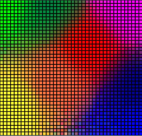
where each point is associated with large dimensional vector, and vectors with similarity are associated with neighbor points. The dimensionality of the map is not related to dimensionality of vectors. In case of text categorization the vectors are rows in document-term table (with sizes near 50,000) and map is one dimensional image like the one shown below

Adjacent points are related documents. The categories may be marked in different colors and we may observe smooth transition from one category to another. So SOM in text categorization is simply the way of sorting documents and graphical representation of results.
Computational part is elementary although many things in it can be optional. I can show the whole process on the tiny example. The starting point is preparation of document-term matrix and random map matrix, which may look for tiny data set like the tables below.
| Data | ||||
|---|---|---|---|---|
| doc/term | w1 | w2 | w3 | w4 |
| d1 | 1.00 | 0.10 | 0.00 | 0.00 |
| d2 | 1.00 | 0.05 | 0.05 | 0.00 |
| d3 | 0.00 | 0.02 | 0.08 | 1.00 |
| d4 | 0.00 | 0.10 | 0.10 | 1.00 |
| Map | ||||
|---|---|---|---|---|
| #/# | 1 | 2 | 3 | 4 |
| 1 | 0.12 | 0.34 | 1.00 | 0.32 |
| 2 | 1.00 | 0.27 | 0.07 | 0.43 |
| 3 | 0.05 | 1.00 | 0.20 | 0.30 |
| 4 | 1.00 | 0.11 | 0.03 | 0.09 |
The data and map tables are normalized, max element in each row equals to 1.00. In a processing step we choose any document row from data table (let say d1) and find closest row in a map table. The proximity measure can be optional. I simply used inner product. For d1 the closest row from map table is #2. After we found it, we correct it by adding difference between d1 and #2 multiplied by coefficient delta:
#2 = #2 + delta * (d1 - #2)
After some experimenting I assigned delta = 0.2. After re-computation
1.00 0.23 0.06 0.34
the map row #2 is replaced. The adjacent rows are also corrected but with lower delta, which achieved by introduction of a value called decay = 0.7.
#row = #row + delta * decayn * (d1 - #row)
where n is distance from the current #row to found best match. Each row in the map is normalized after recalculation. As it may be already clear, we repeat the same step for all rows in data matrix to the end and start it again from the top, until we reach some stable point, where found best matches for each data row stay the same.
The result of the computation is position in the map for each data row in document-term matrix. For PATENTCORPUS128 it looks like these figures below:
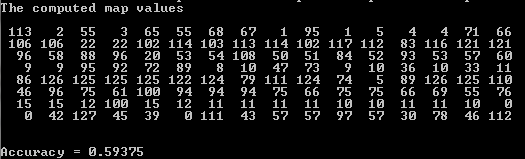
Each row in result is the list of positions in the map for the same category. The accuracy is computed as number of positions sitting within certain range. For example, second row shows that documents from 16 to 31 are associated with map positions mostly from 102 to 117 and few are out of this range 22, 83, 121. Those that are far (22, 83, 121) are considered as wrong mapping the others are considered as right. The accuracy varies, but on average it is between 55 and 65 percent, which is not bad and close to other technologies tested on this site.