Elementary C# (below 400 lines) demo of concept of Random Forest
DEMO of categorization of documents for PATENT CORPUS 128
Random Forest
The algorithm was developed by Leo Breiman and Adele Cutler in the middle of 1990th. Usually, the data to be categorized is known in the form of vectors and the process of categorization is navigation of each vector down along the binary tree, where special condition is applied at each node for choosing left or right direction: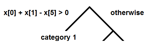
The estimated category is sitting at the bottom branch of the tree and is identified when this branch is reached. The word 'forest' in the name is used because categorization is decided not by the single tree but by the large set of trees called forest. And, if trees provide different categories, the right one is selected as mode value. The word 'random' in the name is used because the nodes and switching conditions are created at a construction by using random sampling from the training set. This is also true for this particular condition shown in the picture X[0] + X[1] - X[5] > 0. It has to be created at a construction for particular group of training vectors and their components randomly but non-the-less navigating to the direction that can provide right categorization when applied for the data. Such condition is called classifier and is the most important part of the algorithm, critical for its efficiency, but not very well explained in papers. Obviously, usage of already created random forest is trivial but the construction of classifiers needs further explanation. Here we suggest technique of making classifiers that is effective for categorization of documents and not necessarily for anything else, like medical symptoms, for example.
Scientific way of making classifiers
During construction time at a particular node we have set of vectors with known categories. These vectors are rows or columns from document/term matrix. In order to make classifier, we simply need to design vector that maximize inner products of one group and minimize inner products of another group of vectors. When vector is found we can distinguish one group from another by assigning conventional border between them. For example, let us look at the following matrix2 3 4 1 0 0 0 1 0 0 3 5 7 3 0 0 0 0 0 0 0 1 1 0 8 9 6 3 3 5 0 0 0 0 4 8 5 3 6 4We can see that top two rows have similarities and statistically different from bottom two rows. This is close to scenario of different vocabulary in different categories. The numbers are simply counts for different words. Obviously, for this case, vector
0 0 0 0 1 1 1 1 1 1is the answer. Its inner products with upper two vectors are 1 and 0, and with bottom two are 34 and 30. We presume that during categorization stage, categorized vector will have similarities either with upper two vectors or with lower two and be categorized correctly. To have such perfect data is obviously wishful thinking, the real data will have noise and classifier has to be found in an optimal way, for example by using ridge regression or support vector machine. At this point I can suggest also method of successive approximations. Let us denote data matrix as D and wanted vector as x. We may introduce known solution for D * x as vector y with small upper two elements and large enough bottom two elements. The least squares solution
x = (DTD)-1 DT y
obviously does not exist or may return random numbers. Adding ridge regression parameter
x = (DTD + k * I)-1 DT y
may return stable solution but the size of D may be as large as 50,000. Making over 1000 nodes is computationally expensive. The answer is to make few iterations for equation
xi+1 = k * DT[ D xi - y] + xi
where k is multiplier that provides computational stability. Initial approximation x0 could be a sum of vectors in one category.
Elementary way of making classifiers
We can reduce the construction of classifies to the following few steps:- identify the category with largest number of vectors
- merge these vectors together in one vector (just add all components)
- find the cosine between this merged vector and each vector in the sample
- take average for smallest and largest cosine value
The last detail to explain is where is the randomness in this algorithm. The construction of each tree starts from the first random sample of vectors taken from the training set. The recommended size of this sample is about 63%. Samples are taken with return. Since size of the training set is, usually, large (100 and more), the number of different samples is large enough to provide as many trees as regular computer can handle for reasonable time. As it, may be clear already, the process of building each tree represents creation of nodes, making classifiers, splitting vectors by using constructed classifies into left and right groups and continue with each group further down until only one vector is left or until all vectors belong to same category. The question that may be asked at this point is why not to make classifiers completely random? This may work with something else but not with classification of text documents. When we make classifier for the group of vectors, we know their categories. It is not wise to ignore information that can be easily used. It is presumed that each individual tree may not be perfect but the whole forest provides good categorization. The details, not mentioned in the article, can be found in elementary demo (below 400 lines) at the top link.
Application of random forest to categorization of real text documents showed accuracy about 65 percent for PATENT CORPUS 128. The project can be downloaded from the second link at the top.